In the previous section we tabulated the values of fx. Now we will tabulate the values of q. For this we use Eq.13.1.
Eq.13.1: q = VQ/Ib
The values are given in table 13.3 below:
Eq.13.1: q = VQ/Ib
The values are given in table 13.3 below:
Table 13.3: Values of q
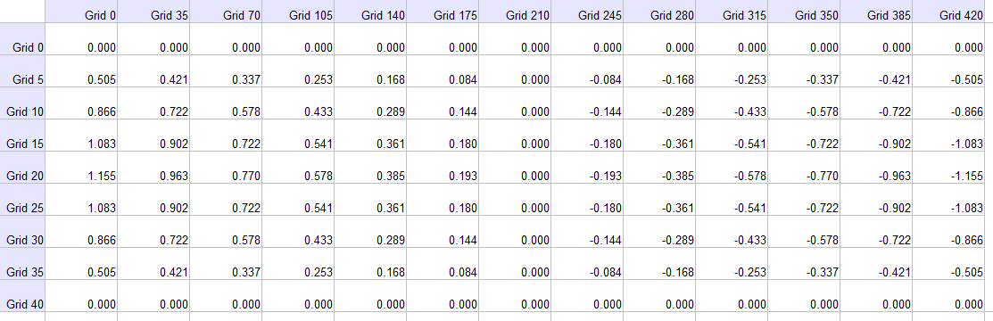
Sample calculation:
Let us take the particle at the intersection of Grid 70 and Grid 35.
From table 13.1, V =30.8 KN.
To find Q :
• Area of the portion above the layer at grid 35 = 0.15 x 0.35 = 0.0525 m2
• Distance of the centroid of this area from the NA = 0.20 - 0.175 = 0.025 m
• So moment of this area about the NA = Q = 0.0525 x 0.025 = 0.0013125 m3
• Moment of inertia of the whole section = = 0.0008 m4
• Width of the section = b =150 mm = 0.15 m
• Substituting these values in eq.13.1 we get, q = 336.875 kN/m2
• This is equal to 0.337 N/mm2 .
In the above table, the following points can be noted:
• The values are symmetric about the Grid 210, as this grid line marks the midpoint of the beam. The values to the right are all negative. This is because the SF here is negative as can be seen from table 13.1
• The values are symmetric about the Grid 20, as this grid line marks the NA. The maximum value in each vertical grid is at the NA. This is in confirmation with the shear stress distribution which we saw earlier in fig.13.3
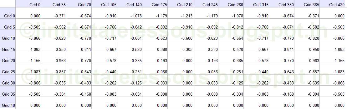
Next we calculate the principal stress f1 in each of the particles. The principal stress f1 is calculated using Eq.13.5 that we saw earlier:
Eq.13.5:Next we calculate the principal stress f1 in each of the particles. The principal stress f1 is calculated using Eq.13.5 that we saw earlier:
Table 13.4. Values of f1:

Sample calculation:
Let us take the particle at the intersection of grid line 30 (horizontal) and grid line 280 (vertical). From table 13.2, fx = 0.539. From table 13.3, q = -.289
Substituting these values in 13.5 we get f1 = 0.664 N/mm2 .
The following points can be noted from the above table:
• The values are symmetric about the Grid 210, as this grid line marks the midpoint of the beam.
• The values are not symmetrical about the Grid 20 grid line which marks the NA)
• All the values are positive. This indicates that f1 is tensile in nature.
• The maximum value in each vertical grid is at the NA. Among these maximum values at the NA, the ones at the supports are the largest.
Now we calculate the principal stress f2 . For this we use Eq.13.7
Eq.13.7
The values of f2 calculated using Eq.13.7 are given in table 13.5 below:
Table 13.5. Values of f2:
Sample calculation:
Let us take the particle at the intersection of grid line 15 (horizontal) and grid line 35 (vertical). From table 13.2, fx = -0.093. From table 13.3, q = .902
Substituting these values in 13.5 we get f2 = 0.950 N/mm2 .
• The following points can be noted from the above table:
• The whole table is a mirror reflection of the previous table 13.4
• The values are symmetric about the Grid 210, as this grid line marks the midpoint of the beam.
• The values are not symmetrical about the Grid 20 grid line which marks the NA)
• All the values are negative. This indicates that f2 is compressive in nature.
• The maximum value in each vertical grid is at the NA. It is numerically equal to q. Among these maximum values at the NA, the ones at the supports are the largest.
From the above two tables 13.4 and 13.5, we can see that tensile stresses and compressive stresses exists on various portions of the body of the beam. When we learned about the 'Design for flexure' in the previous chapters, we discussed the effect of 'bending moment' on the beam. There we provided steel to resist the tensile forces formed due to those bending moments. But here we just saw that tensile forces are produced not only due to the bending moments, but also due to shear forces. (The compressive forces in table 13.5 is of not much significance when we consider a concrete beam because concrete is strong in compression). So we have to learn more about these tensile forces.
Let us calculate the angle made by plane PQ with the vertical. We have seen that this angle (denoted as α ) is obtained using Eq.13.6
Eq.13.6:
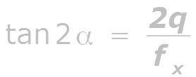
Table 13.6. Values of α:
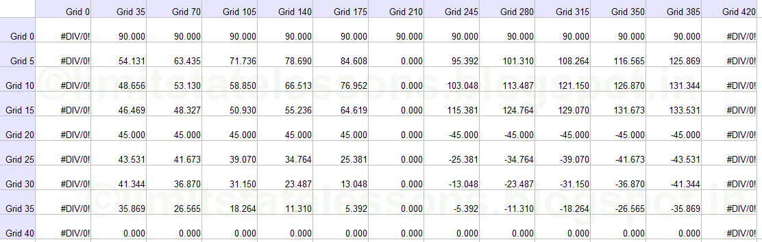
Sample calculation:
Let us take the particle at the intersection of grid line 35 (horizontal) and grid line 70 (vertical). This particle has some symmetric points above the NA (Grid line 20) and also on the other side of the midpoint of the beam (Grid line 210). In the next section we will see these particular points.
Copyright ©2015 limitstatelessons.blogspot.com - All Rights Reserved
No comments:
Post a Comment